Uniform Distribution

The Uniform distribution is one of the simplest continuous probability distributions. It describes a scenario where all outcomes within a certain range are equally likely. It is often used when there is no prior knowledge favoring one outcome over another within the defined range.

Probability Density Functions (PDF)

If X∼U(a,b), where:

• a: Minimum value (lower bound),
• b: Maximum value (upper bound),

then the PDF is given as:

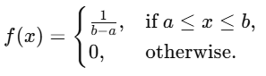
Cummulative Density Function (CDF)

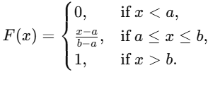
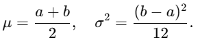
Mean & Variance

The mean and variance are:

Applications of Uniform Distribution in Healthcare

1. Medical Device Calibration: Suppose a medical device produces measurements uniformly distributed within a range. The distribution can be used to assess expected readings.
2. Patient Arrival Times: The time intervals between patient arrivals at a clinic are uniformly distributed during specific hours.

For the Uniform distribution:

• The PDF is constant: f(x)=1/(b−a).
• The probability of a specific value (e.g., P(X=20)) is also zero, because there is no width (interval) to calculate the area.

Unlike the Normal distribution, where the density varies, the Uniform distribution’s density is constant.

Problem

A hospital measures the waiting times of patients at a diagnostic center, which are uniformly distributed between 10 minutes and 30 minutes. Calculate:

1. The probability that a patient waits less than 15 minutes.
2. The probability that a patient waits more than 25 minutes.
3. The mean and variance of the distribution.

Parameters:

• a=10a = 10a=10 (minimum wait time),
• b=30b = 30b=30 (maximum wait time).

1. Probability that X<15(CDF):

P(X < 15) = F(15) = (15 − 10)/(30 − 10) = 5/20 = 0.25

2. Probability that X>25 (Complement Rule):

P(X > 25) = 1 − P(X ≤ 25)
P(X ≤ 25)=F(25)=(25 − 10)/(30 − 10) = 15/20 = 0.75
P(X > 25)=1−0.75=0.25

3. Mean and Variance:

μ = (a + b)/2 = (10 + 30)/2 = 20 minutes.
σ² = (b − a)²/12 = (30 − 10)²/12 = 400/12 = 33.33 (minutes squared).

Calculating using R

# Parameters

> a <- 10 # Minimum waiting time
> b <- 30 # Maximum waiting time

# 1. Probability that a patient waits less than 15 minutes

> prob_less_than_15 <- punif(15, min = a, max = b)
> prob_less_than_15

# 2. Probability that a patient waits more than 25 minutes

> prob_greater_than_25 <- 1 – punif(25, min = a, max = b)
> prob_greater_than_25

# 3. Mean and variance

> mean <- (a + b) / 2
> variance <- (b – a)^2 / 12
> mean
> variance