Data frames are one of the most widely used data structures in R. They allow you to store tabular data in rows and columns, making them ideal for working with datasets. A data frame is a two-dimensional, tabular data structure in R where each column can have a different type (e.g., numeric, character, factor). It is similar to a table in SQL or a dataframe in Python.
Creating data frame: Use data.frame() to create a data frame. You can also convert other objects (like lists or matrices) into data frames using as.data.frame().
Please note: Use Control + Shift + A by clicking the line number. This allows your code to get formatted and make it easier working on lengthier codes. You can alternatively go to ‘Code‘ menu in R Studio & click on ‘Reformat code‘.
Functions to explore the structure and metadata of a data frame:
> str(friend_data) # Displays the structure of the data frame > class(friend_data) # “data.frame” – Class of the object > dim(friend_data) # Dimensions – number of rows and columns > nrow(friend_data) # Number of rows > ncol(friend_data) # Number of columns > colnames(friend_data) # Column names > rownames(friend_data) # Row names > attributes(friend_data) # Attributes of the data
Accessing Data in a Data Frame: By columns
> friend_data$friend_name # Access the “friend_name” column > friend_data[, 2] # Using column indexing – access the second column > friend_data[[“friend_name”]] # Using column name indexing > friend_data[, c(“friend_name”, “friend_age”)] # Selecting multiple columns
Accessing Data in a Data Frame: By rows
> friend_data[1, ] # First row > friend_data[c(1, 3), ] # First and third rows > friend_data[-1, ] # All rows except the first
Subsetting Rows and Columns
> friend_data[friend_data$friend_age > 25, ] # Rows based on condition – Friends older than 25 > friend_data[1:2, c(“friend_name”, “friend_age”)] # Specific rows and columns
> friend_data$friend_city <- NULL > friend_data <- friend_data[, -2] # Exclude columns using negative indexing – Remove second column
Visualizing first and last few rows
> head(friend_data) # default six rows > head(friend_data, 2) # First two rows > tail(friend_data) # default six rows > tail(friend_data, 2) # Last two rows
Summary of the data – basic descriptive statistics > summary(friend_data)
Unique Values: > unique(friend_data$friend_name)
Sort: > friend_data <- friend_data[order(friend_data$friend_age), ] # Ascending by age
Verfiying missing values:
> any(is.na(friend_data)) # TRUE/FALSE for any missing values > which(is.na(friend_data)) # Positions of missing values
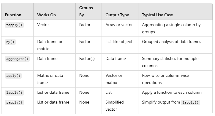
Grouped Aggregation with split() – splits a vector or data frame into groups based on a factor and applies a function to each subset.
> split_data <- split(mtcars, mtcars$cyl) # Split mtcars data by cylinder type > avg_mpg <- sapply(split_data, function(group) mean(group$mpg)) print(avg_mpg) # Calculate avg mpg for each group
Table-Based Aggregation – table() & prop.table() creates contingency tables for counts, proportions, and cross-tabulations.
> cyl_count <- table(mtcars$cyl) print(cyl_count) # Count of cars by cylinder type > cyl_prop <- prop.table(cyl_count) # proportion of cars by cylinder type > print(cyl_prop)
Aggregating missing data
> data <- data.frame( group = c(“A”, “A”, “B”, “B”, “C”, “C”), value = c(10, NA, 20, 30, NA, 40) ) # Create a sample data frame with missing values > agg_na <- aggregate(value ~ group, data = data, FUN = function(x) sum(x, na.rm = TRUE)) # Aggregating sum ignoring na. > print(agg_na)