
The Normal Distribution, also known as the Gaussian Distribution or bell curve, is one of the most important and widely used probability distributions in statistics. Four main reasons for this – the distribution is very tractable analytically, the distribution with its bell shape and symmetry makes it compelling choice for population models, this distribution as per Central Limit Theorem can be used to approximate a large variety of distributions in large samples and finally the mathematical properties are simple. It describes a continuous probability distribution for a random variable. The distribution is symmetrical, with most of the observations clustering around the central peak and the probabilities for values tapering off equally in both directions from the mean.
Probability Density Function (pdf)
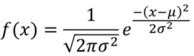
The parameters for normal distribution are mean (µ) and variance (σ2). The PDF is used to find the likelihood of a continuous random variable falling within a particular range of values. For example, predicting the likelihood of a person having a certain height.
The pdf is given as:
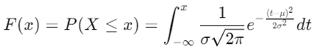
Cumulative Density Function (CDF)
The CDF is used to calculate probabilities for ranges of values and is often used in hypothesis testing and confidence interval estimation. The cdf is given as:
These functions can be calculated in R easily.
R Functions for Normal Distribution: pnorm, dnorm, qnorm
- dnorm(x, mean, sd): Computes the “density not probability” PDF of the normal distribution at a specific value x with given mean and standard deviation.
Usage: To find the density (height of the curve) at a particular value of x.
- pnorm(q, mean, sd): Computes the “probability” CDF of the normal distribution up to a specific value q with given mean and standard deviation.
Usage: To find the probability that a random variable is less than or equal to q.
- qnorm(p, mean, sd): Computes the quantile function (inverse of CDF) of the normal distribution for a given probability p.
Usage: To find the value q such that the probability of the variable being less than or equal to q is p.
Properties of Probabilities in a Normal Distribution
For any normal distribution with mean μ and standard deviation σ:
- Complement Rule: This property is useful when you want the probability of a value being greater than a certain point, which is the complement of the cumulative probability up to that point.
P(X>a) = 1 − P(X≤a) - Symmetry: The normal distribution is symmetric around its mean, μ. Thus: P(X>μ+k) = P(X<μ−k); for any value k.
- Between Two Values: For probabilities between two values, a and b: P(a<X≤b) = P(X≤b) − P(X≤a) This is the difference between the cumulative probabilities up to b and a.
- Standard Normal Distribution: If Z is a standard normal variable (mean = 0, standard deviation = 1): P(Z>z) = 1 − P(Z≤z)
- Tail Properties: For the left tail:
P(X<a) = P(X≤a); because it is continuous.
For the right tail: P(X>a) = 1 − P(X≤a)
Problem Solving
Let us work on a problem with mtcars/mpg.
First, we find the mean & standard deviation. We will work on mtcars data in R.
> data(mtcars)
> mean(mpg) # 20.09062
> sd(mpg) # 6.026948
If we want to calculate the pdf for an exact value say 21 mpg.
> dnorm(21, 20.09062, 6.026948)
We get 0.06544387. The Probability Density Function (PDF) provides the relative likelihood of a continuous random variable taking a specific value.
The PDF tells you how likely it is to observe a value close to a specific x. For instance, if the PDF value at x = 21 is high, it means that an MPG value of 21 is more probable compared to other values. However, we got a lower probability (0.065…) so 21 is less probable compared to other values. While the mean gives you a single summary statistic, the PDF gives you a complete picture of how your data is distributed.
To find the probability that MPG is less than a specific value, we use the CDF. For example, between 20 & 25.
> pnorm(25, 20.09062, 6.026948) – pnorm(20, 20.09062, 6.026948)
We get 0.2983394 ~ 0.30. The interpretation here is that there is only 30% chance that the value for MPG falls between 20 & 25.
Similarly, if you want to find the probability for MPG that is less than a specific value for x then we use pnorm.
> pnorm(21, 20.09062, 6.026948)
Again, if you want to find the probability for mpg that is greater than a specific value say 21 the we use
1 – pnorm(21, 20.09062, 6.026948)
We get 0.440033 ~ 44% chance that the mpg will take the value greater than 21. Why? Because P(X>21) = 1−P(X≤21).
To calculate probabilities for values greater than a specific point in a normal distribution, the pnorm function is used in conjunction with the complement rule (1 – pnorm(…)). This approach is commonly used in hypothesis testing and other statistical analyses to understand the likelihood of observing values in the tails of a distribution.
Lets say we want to calculate the threshold above which 5% of the data lies in a normal distribution. In this case, we use qnorm as we want to find the 95th percentile of a standard normal distribution.
> qnorm(0.95, mean = 0, sd = 1)
Let us say you want to experiment with a sample generated from a normal distribution.
For random number generation you will use rnorm.
> set.seed(123) # use this whenever you want reproducibility.
> rnorm(100, mean = 0, sd = 1)
The rnorm function here generates 100 random numbers from standard normal distribution.
A company manufactures light bulbs, and the lifespan of these bulbs is normally distributed with a mean (μ) of 800 hours and a standard deviation (σ) of 50 hours. Using this info:
1. Calculate the probability density function (PDF) at 850 hours.
> dnorm(850, 800, 50)
This value is not a probability but a density and provides a sense of how likely values around 850 are compared to other values.
2. Find the cumulative distribution function (CDF) for bulbs lasting less than 850 hours.
> pnorm(850, 800, 50)
The result gives the cumulative probability that a bulb lasts less than or equal to 850 hours.
3. Determine the probability that a bulb lasts more than 850 hours.
Use complement rule; P(X>850) = 1−P(X≤850)
> 1 – pnorm(850, 800, 50)
The probability of a bulb lasting more than 850 hours is simply 1−P(X≤850).
4. Calculate the probability that a bulb lasts between 750 and 850 hours.
P(750<X≤850) = P(X≤850) − P(X≤750)
> pnorm(850, 800, 50) – pnorm(750, 800, 50)
This gives the probability that the lifespan of the bulbs falls between 750 and 850 hours.