A t-test is a type of inferential statistic used to determine if there is a significant difference between the means of two groups, which may be related in certain features. It helps assess whether the observed difference between the sample means is due to chance or reflects a true difference in the population. The t-test is especially useful when:
- The sample size is small (typically n<30).
- The population standard deviation is unknown.
The t-test is a versatile and widely used method for comparing means between groups. It is essential in situations with small sample sizes or when population parameters are unknown.
Why We Use t-Tests?
The primary reason for using a t-test is to compare two means to see if they are statistically different from each other. This could be comparing:
- The mean of a sample against a known value (one-sample t-test).
- The means of two independent groups (independent t-test).
- The means of paired groups (paired t-test).
A t-test is useful in many real-world scenarios, including:
- Medicine: Testing whether a drug is more effective than a placebo.
- Education: Assessing whether a new teaching method improves test scores.
- Marketing: Comparing sales data before and after a marketing campaign.
Types of t-Tests
1. One-Sample t-Test:
Compares the mean of a single sample to a known value.
Example: Comparing the average test score of a group of students to the national average.

Where x̄ is the sample mean, μ is the population mean, s is the sample standard deviation, and n is the sample size.
2. Independent Two-Sample t-Test:
Compares the means of two independent groups (e.g., control vs. experimental group). Assumes that the two groups are not related.

Where x̄1 and x̄2 are the sample means, s12 s22 are the variances of the groups, and n1, n2 are the sample sizes.
3. Paired t-Test:
Compares two measurements taken from the same individual or related groups (e.g., before and after treatment). The focus is on the difference in means for paired observations.

Where đ is the mean of the differences between paired observations, sd is the standard deviation of the differences, and n is the number of pairs.
Difference Between Paired & Two-Sample t-Test
A two-sample t-test compares the means of two independent groups (e.g., treatment vs. control), while a paired t-test compares two related observations (e.g., measurements on the same subjects before and after treatment).
How the t-Test Works?
When performing a t-test, you are essentially asking: “Is the difference between group means large enough to suggest that the two groups come from different populations?”
- Null Hypothesis (H₀): The null hypothesis states that there is no significant difference between the means (e.g., μ1=μ2 for two groups, or μ=μ0 for one group).
- Alternative Hypothesis (H₁): The alternative hypothesis claims that there is a significant difference between the means (e.g., μ1≠μ2).
- t-Statistic: The t-statistic is calculated based on the difference between sample means, taking into account the variability in the data and the sample size. A larger t-statistic means that the difference is more likely to be statistically significant.
- Degrees of Freedom (df): The degrees of freedom reflect the number of independent values in your data that are free to vary. For a simple t-test, df=n−1, where n is the sample size.
- p-Value: After calculating the t-statistic, you compare it to a critical value from the t-distribution, which gives you a p-value. The p-value indicates the probability of observing such an extreme result if the null hypothesis were true.
- If the p-value is less than the significance level (e.g., α=0.05), you reject the null hypothesis, meaning there is enough evidence to support a significant difference.
- If the p-value is greater than α, you fail to reject the null hypothesis, meaning the evidence does not support a significant difference.
Testing assumptions for the t-test
- Normality: The data should be approximately normally distributed. For large samples, the Central Limit Theorem ensures that the distribution of the sample mean will be approximately normal, even if the data are not.
- Independence: The observations should be independent of each other. For a two-sample t-test, this means the two groups should not influence each other.
- Equal Variances: For an independent two-sample t-test, it is assumed that the variances in the two groups are equal (homoscedasticity). If this is not true, you may need to use Welch’s t-test, which does not assume equal variances.
When to Use a t-Test?
- Small Sample Sizes: If your sample size is small (less than 30), the t-test is ideal.
- Unknown Population Standard Deviation: When the standard deviation of the population is unknown, the t-test is preferred over the z-test, which requires knowledge of the population standard deviation.
- Comparing Means: If your research question involves comparing the means of two groups or comparing a sample mean to a known value.
Let us look at how one-sample and two-sample t-tests can be applied in the pharmaceutical industry, which often revolves around the testing and effectiveness of drugs or treatments.
Problem 1: One-Sample t-Test (Drug Dosage)
A pharmaceutical company is developing a new blood pressure medication. The company claims that the average reduction in systolic blood pressure after taking the drug is 20 mmHg. To verify this claim, the company tests the drug on a small sample of patients.
The data collected from a sample of 10 patients shows the following reductions in systolic blood pressure:
reduction: [18,22,19,21,20,17,24,19,18,20]
The company wants to test if the true mean reduction is significantly different from 20 mmHg, at a significance level of 0.05.
Step 1: Stating the Hypothesis
Null Hypothesis (H₀): The true mean reduction in blood pressure is 20 mmHg.
H0: μ = 20
Alternative Hypothesis (H₁): The true mean reduction is different from 20 mmHg.
H1: μ ≠ 20
Step 2: Calculations using R
> bpred <- c(18, 22, 19, 21, 20, 17, 24, 19, 18, 20)
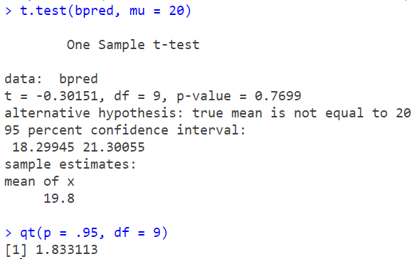
> t.test(bpred, mu = 20)
> qt(p = .95, df = 9)
Step 3: Interpretation & Results
The t-statistic will measure how far the sample mean is from 20 mmHg. If test statistic t > tcrit, df=9, we reject the null hypothesis and conclude that the true mean reduction is significantly different from 20 mmHg.
The p-value will help determine whether the observed difference is statistically significant. If the p-value < 0.05, we reject the null hypothesis and conclude that the true mean reduction is significantly different from 20 mmHg.

The p-value (0.769) > 0.05, we fail to reject null. This means that the true mean is not significantly different from 20 mmHg. This indicates that no effect was observed.
Problem 2: Two-Sample t-Test (Drug Efficacy Between Two Groups)
A pharmaceutical company is testing two different formulations of a drug intended to reduce cholesterol levels. The company wants to compare the effectiveness of Formulation A and Formulation B in reducing cholesterol levels after 8 weeks.
- Group A (Formulation A): [18, 22, 19, 23, 20, 21, 24, 20]
- Group B (Formulation B): [25, 29, 24, 28, 27, 26, 31, 29]
Step 1: Hypothesis
The company wants to test whether there is a significant difference in the cholesterol reduction between the two formulations. Null Hypothesis (H₀): There is no significant difference in cholesterol reduction between the two formulations.
H0: μA = μB
Alternative Hypothesis (H₁): There is a significant difference in cholesterol reduction between the two formulations.
H1: μA ≠ μB
Step 2: Calculations
> formulaA <- c(18, 22, 19, 23, 20, 21, 24, 20)
> formulaB <- c(25, 29, 24, 28, 27, 26, 31, 29)
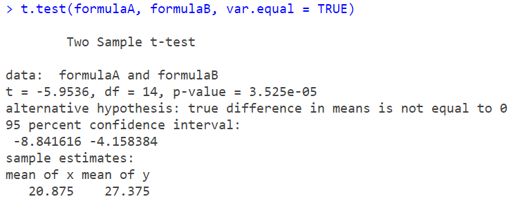
> t.test(formulaA, formulaB, var.equal = TRUE)
Step 3: Interpretation & Results
The t-statistic will help compare the means of the two formulations.
The p-value will tell if the difference between the formulations is statistically significant. If the p-value < 0.05, we reject the null hypothesis and conclude that there is a significant difference in efficacy between the two drug formulations.

> format(3.525e-05, scientific = FALSE) # 0.00003525
The p-value < 0.05, we reject null. There is a significant difference in efficacy between the two drug formulations A & B.
Problem 3: Paired t-test (Before & After)
A pharmaceutical company tests the efficacy of a new drug by measuring patients’ blood pressure before and after the drug is administered. Each patient’s measurements are paired, as the before-and-after measurements are dependent on the same person.
before – 140, 150, 160, 130, 145
after – 135, 140, 155, 125, 138
Step 1: Hypothesis
Null Hypothesis (H₀): The mean difference between before & after blood pressure measurements is zero.
H0: μd=0
Alternative Hypothesis (H₁): The mean difference between the before and after measurements is not zero.
H1: μd≠0
Step 2: Calculation using R
Since p=0.0054<α=0.05p = 0.0054 < \alpha = 0.05p=0.0054<α=0.05, we reject the null hypothesis (H0H_0H0).
Step 3: Interpretation & Results

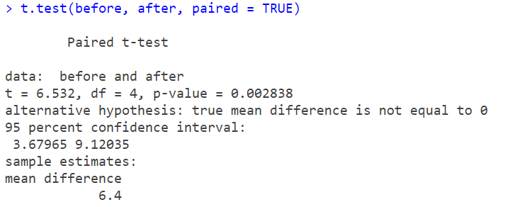
Since p=0.0028<α=0.05, we reject the null hypothesis (H0). There is strong evidence to suggest that the mean difference in blood pressure between the “before” and “after” measurements is significantly different from 0(p=0.0028). The mean difference is estimated to be 6.4, and the true mean difference likely falls between 3.67965 & 9.12035 with 95% confidence. This indicates a significant reduction in blood pressure after treatment.
These types of t-tests are crucial in the pharmaceutical industry for evaluating drug effectiveness, comparing formulations, and supporting claims regarding treatment outcomes.
