Let us work on a problem with 3 groups and use 1-way ANOVA to find significance. Imagine you are a pharmaceutical researcher analyzing the effectiveness of three new drug formulations (Drug A, Drug B and Drug C) designed to lower blood pressure. Three drugs were given to three separate groups of patients, and the blood pressure was recorded for each patient.
Group 1: drugA – 120, 115, 123, 130, 117
Group 2: drugB – 110, 105, 112, 115, 107
Group 3: drugC – 100, 98, 105, 110, 102
You want to know if there is a significant difference in average blood pressure reduction between the groups. ANOVA will help you compare all three groups simultaneously.
1. State the hypothesis
- H₀: The mean blood pressure reduction for all three groups is the same i.e.,
H₀: μ₁ = μ₂ = μ₃. - H₁: At least one group has a significantly different mean blood pressure reduction i.e.,
H₁: At least one mean differs.
2. Create vectors & data frames in R
library(ggplot2)
library(dplyr)
drugA <- c(120, 115, 123, 130, 117)
drugB <- c(110, 105, 112, 115, 107)
drugC <- c(100, 98, 105, 110, 102)
drugeff <- data.frame(bp = c(drugA, drugB, drugC), drug = factor(rep(c(“A”, “B”, “C”), each = 5)))
3. Calculate mean & CI
summary_data <- drugeff %>%
group_by(drug) %>%
summarise(
mean_bp = mean(bp),
sd_bp = sd(bp),
n = n(), se = sd_bp / sqrt(n), # Standard Error
ci_lower = mean_bp – qt(1 – 0.05 / 2, n – 1) * se, # Lower 95% CI
ci_upper = mean_bp + qt(1 – 0.05 / 2, n – 1) * se # Upper 95% CI
)
4. Visualize mean using bar plot with error bars
ggplot(summary_data, aes(x = drug, y = mean_bp)) +
geom_point(size = 3) + # Mean points
geom_errorbar(aes(ymin = ci_lower, ymax = ci_upper), width = 0.2) + # Error bars for CI
labs(title = “Mean Blood Pressure Reduction with 95% Confidence Intervals”,
x = “Drug”,
y = “Blood Pressure Reduction (mmHg)”) +
theme_minimal()

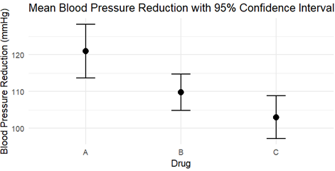
The width (and the presence of outliers) shows how much variation there is within each group. A wider group means more variability in reduction within that group. We can see group A is wider with no outlier.
The middle point inside each group gives the mean reduction for each drug. If one drug has a much higher mean than another, it suggests that drug is more effective. Here, Drug A seems to be more effective comparted to the rest.
If the boxes are clearly separated with minimal overlap, it suggests that the group means (i.e., drug effects) are likely different, which would support rejecting the null hypothesis in ANOVA (i.e., that all drug means are equal).
If the boxes overlap considerably, it might suggest that the drugs don’t have statistically different effects on blood pressure, which would support failing to reject the null hypothesis. In our case, Drug A & B are separated with minimal overlap whereas Drug B & C overlap considerably suggesting both the drugs do not have statistically different effects on blood pressure.
5. Fitting the model
anova1way <- aov(bp ~ drug, data = drugeff)
We fit the model first that allows us to check for assumptions. A model will have a good fit if the p-value & F-statistic i.e., a low p-value usually < 0.05 indicates statistically significant model which means that the model is capturing a meaningful relationship between independent and dependent variable. Any assumption failure also indicates a poor fit.
6. Test Assumptions
a. Independence
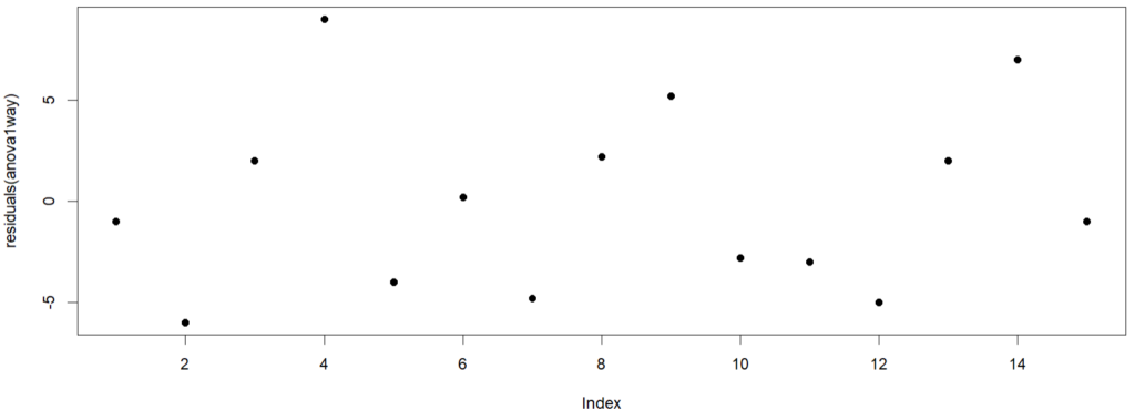
plot(residuals(anova1way), pch = 16)

From the residual plot, we see that the residuals do not cluster together in certain time periods. We do not see any abnormal patterns or trends (upward or downward). The residuals do not repeat a cyclical pattern over time. All these suggests non-independence. We can do a more formal test called the Durbin-Watson test.
Hypothesis (Durbin-Watson test):
H0: Samples are independent
H1: Samples are not independent
Require(car)
durbinWatsonTest(anova1way)

The p-value > 0.05. We fail to reject null. We have sufficient evidence to confirm that the samples are independent of each other.
b. Homoscedasticity (constant variance)
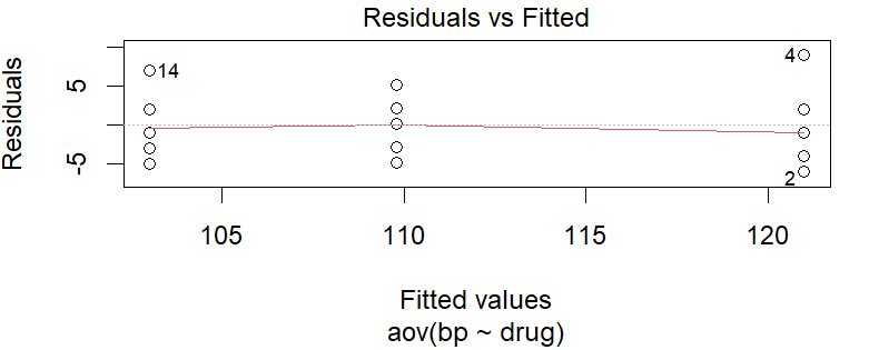
We can plot the residuals vs fitted to visually check for constant variance.
plot(anova1way, 1)

From the residual vs fitted plot, we see random scatter of points around the horizontal line at zero, indicating that the relationship between the variables is linear. The errors (residuals) have constant variance across the range of fitted values. No pattern or trend is visible. All these suggest linearity & equal error variances. To confirm this, we use Bartlett’s test.
Hypothesis (Bartlett’s test):
H0: σ12 = σ22 = σ32
H1: σ12 ≠ σ22≠ σ32
bartlett.test(bp ~ drug, data = drugeff)

The p-value > 0.05. We fail to reject null. We have sufficient evidence to confirm that the variances are not significantly different and the assumption of homogeneity of variance holds.
c. Normality
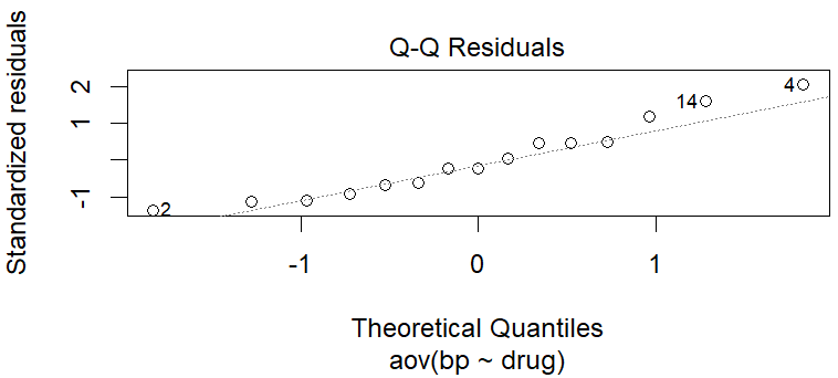
For normality, we visualise using the normal Q-Q plot.
plot(anova1way, 2)

Looking at the Q-Q (Quantile-Quantile)plot, the residuals are normally distributed, the points almost fall roughly along a straight diagonal line (the 45-degree line or the “line of equality”). There seems to be outliers but we can confirm with a formal test.
Hypotheses (Shapiro-Wilk Test):
Null Hypothesis (H0): The residuals are normally distributed.
Alternative Hypothesis (H1): The residuals are not normally distributed.
shapiro.test(residuals(anova1way))

The p-value > 0.05. We fail to reject null. We have sufficient evidence to confirm that the data is normal.
7. Perform one-way ANOVA
summary(anova1way)
Interpretation of the output:

Degrees of freedom (df):
Drug (Between Groups): The degrees of freedom for the drug factor is 2. This corresponds to the number of drug groups minus 1. In your case, you have three drug groups (A, B, C), so the degrees of freedom is 3−1=2.
Residuals (Within Groups): The residual degrees of freedom is 12, which represents the total number of observations minus the number of groups. If you had 15 total observations (5 in each group), then 15−3=12.
Sum of Squares (Sum Sq):
Drug (Between Groups): The sum of squares for the drug factor is 826.1, representing the variability in blood pressure reduction explained by the differences between the drug groups.
Residuals (Within Groups): The sum of squares for the residuals is 288.8, representing the variability within each drug group (i.e., individual differences in blood pressure reduction that are not explained by the drug treatments).
Mean Squares (Mean Sq): Drug (Between Groups): The mean square for the drug factor is 413.1, calculated as the sum of squares divided by the degrees of freedom (826.1 / 2).
Residuals (Within Groups): The mean square for the residuals is 24.1, calculated as 288.8 / 12.
F-value:
The F-value is the ratio of the mean square for the drug factor to the mean square for the residuals: 413.1/24.1 = 17.16.
A higher F-value indicates that there is more variation between the drug groups compared to the variation within the groups.
p-value (Pr(>F)):
The p-value for the drug factor is 0.000302. This is the probability of observing such a large F-value (or a more extreme one) if the null hypothesis were true (i.e., if there were no difference between the drug groups).
Since the p-value is very small (less than 0.05 and even less than 0.001), you can reject the null hypothesis. This means there is a statistically significant difference in blood pressure reduction among the three drug groups.
Significance Codes:
The triple asterisks (***) next to the p-value indicate a high level of statistical significance (p < 0.001). In R’s significance coding, this is the highest level of significance.
One-way ANOVA interpretation:
The ANOVA test suggests that there is a statistically significant difference in blood pressure reduction between at least two of the drug groups (A, B, or C).
However, ANOVA does not tell us which specific drug groups differ from each other. We would use a post-hoc test like Tukey’s HSD.
Conclusion:
Based on this ANOVA result, we conclude that the type of drug has a significant effect on blood pressure reduction. The small p-value (0.000302) indicates that it is highly unlikely that the observed differences in blood pressure reduction between drugs are due to random chance.
Refer Post-Hoc Tukey’s HSD the last step (step 8) for finding the most effective drug.
