The law of large numbers

The Law of Large Numbers (LLN) is a fundamental theorem in probability and statistics that describes the result of performing the same experiment a large number of times. The LLN states that as the number of trials or observations increases, the sample mean will converge to the expected value (population mean) of the underlying random variable. In general, The Law of Large Numbers (LLN) states that as the number of trials (or sample size) increases, the sample mean converges to the population mean.

There are two main versions of the Law of Large Numbers:

Weak Law of Large Numbers (WLLN): States that the sample mean converges in probability towards the expected value as the sample size grows to infinity.

Strong Law of Large Numbers (SLLN): States that the sample mean almost surely converges to the expected value as the sample size grows to infinity. “Almost surely” means with probability 1. Insurance companies rely on the LLN to predict claims. Although they can’t predict the number of claims in a given month, they know that as the number of policyholders increases, the average amount of claims paid out will converge to a predictable number. This allows them to set premiums and reserve amounts accurately. Similarly, Casinos use the LLN to ensure profitability. While the outcome of any single game is unpredictable, over a large number of games, the average payouts will converge to a predictable value, allowing casinos to remain profitable. For example, in roulette, the house edge ensures that over thousands of spins, the casino will win more money than it loses.

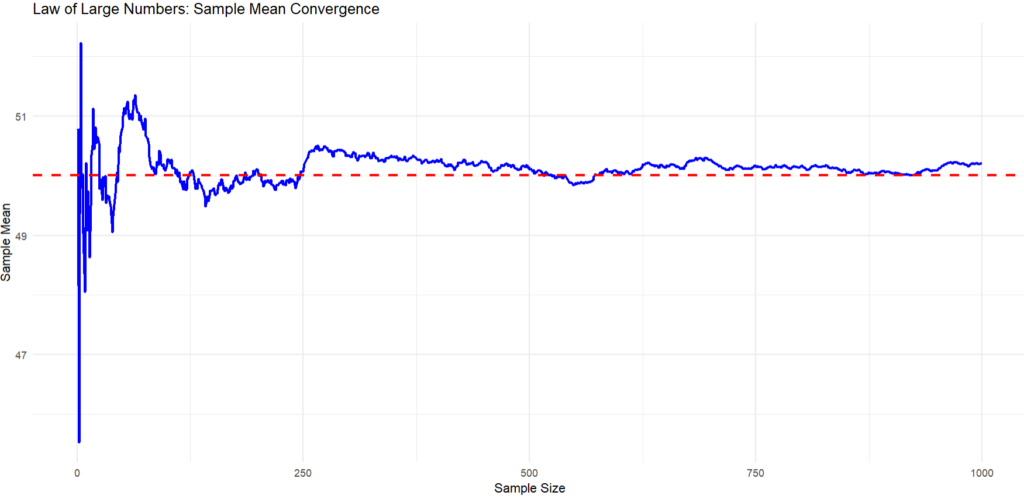
Here is an illustration to understand Law of Large Numbers better:

Load necessary library

> library(ggplot2)

Set seed for reproducibility

> set.seed(123)

Step 1: Simulate a population

> population <- rnorm(100000, mean = 50, sd = 10) # Normal distribution

Step 2: Function to calculate sample means incrementally

> sample_sizes <- 1:1000 # Range of sample sizes
> sample_means <- cumsum(sample(population, size = length(sample_sizes), replace = TRUE)) / sample_sizes

Step 3: Create a data frame for plotting

> lln_data <- data.frame(
sample_size = sample_sizes,
sample_mean = sample_means
)

Step 4: Plot sample mean vs population mean

> ggplot(lln_data, aes(x = sample_size, y = sample_mean)) +
geom_line(color = “blue”, size = 1) +
geom_hline(yintercept = mean(population), color = “red”, linetype = “dashed”, size = 1) +
labs(
title = “Law of Large Numbers: Sample Mean Convergence”,
x = “Sample Size”,
y = “Sample Mean”
) +
theme_minimal()

What we see in the plot?

1. The red dashed line indicates the true population mean.
2. We see the blue line (sample mean) fluctuates significantly for small sample sizes. As the sample size increases, the sample mean stabilizes and approaches the red line (population mean).
3. This shows the convergence of the sample mean to the population mean as the sample size increases.

What is the difference between CLT & LLN?

While both the CLT and LLN are related to the behaviour of sample means, they focus on different aspects:

CLT explains the shape of the sampling distribution (it becomes normal).

LLN explains the convergence of the sample mean to the population mean.