Measures of shape, describe the distribution of data within a set. They can assist find potentially hidden patterns in data and are frequently used to detect non-normality. The two main measures of shape are skewness and kurtosis.
Symmetry and Skewness
Skewness is a measure of the degree of asymmetry of a distribution of random variables about its mean.

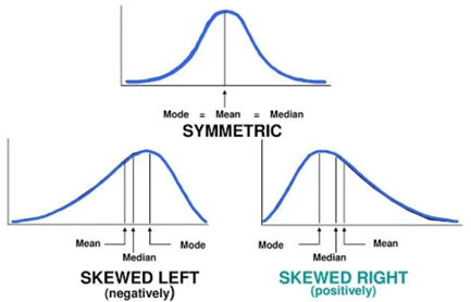
A distribution is said to be right-skewed (or positively skewed) if the right tail seems to be stretched from the center. A left-skewed (or negatively skewed) distribution is stretched to the left side. A symmetric distribution has a graph that is balanced about its center.

> library(e1071) # or use library(moments)
> skewness(mtcars$mpg
The sample skewness (g1) ranges from -1 to 1. If g1 > 0 indicates right-skewed distributions (positively skewed), while g1 < 0 indicates left-skewed distributions (negatively skewed). The values of g1 approaching zero suggest a symmetric distribution.
How do we determine if an observed value of g1 is “big” enough to be considered skewed to the right or left? A decent rule of thumb is that if g1 > 2(sqrt(6/n)) are significantly skewed in the direction of the sign of g1.
A normal distribution has a bell-shaped, symmetric curve where:
- The mean, median, and mode are equal.
- The data is symmetrically distributed around the center.
- 68% of the data lies within 1 standard deviation, 95% within 2, and 99.7% within 3 standard deviations.
In case of a skew
If the mean < median, negative/left skewed/long tail on the left
If the mean = median, symmetrical
If the mean > median, positive/right skewed/long tail on the right
Kurtosis
Another component to the shape of a distribution is how “peaked” it is.

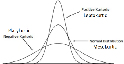
Some distributions tend to have a flat shape with thin tails. These are called platykurtic, and an example of a platykurtic distribution is the uniform distribution. On the other end of the spectrum are distributions with a steep peak, or spike, accompanied by heavy tails; these are called leptokurtic. In between are distributions (called mesokurtic) with a rounded peak and moderately sized tails. The standard example of a mesokurtic distribution is the famous bell-shaped curve, also known as the Gaussian, or normal, distribution.

> library(e1071) # or library(moments)
> kurtosis(mtcars$mpg)
The samples with g2 > 0 are called leptokurtic, and samples with g2 < 0 are called platykurtic. Samples with g2 = 0 are called mesokurtic.
